Introduction to Pandas
What is Pandas?
Pandas is a popular Python library that offers high-performance and easy-to-use data manipulation and analysis tools. It is a go-to library for working with structured and semi-structured data such as tables and time-series data. Pandas provides a wide range of functions and data structures that allow data scientists, analysts, and researchers to quickly clean, transform, and manipulate data to extract meaningful insights.
Why Pandas? (1)
Efficient Handling of Tabular Data: Pandas can efficiently handle tabular data, enabling users to work with data from various file formats like CSV, Excel, SQL databases, and more.
Support for Huge Datasets: Pandas is designed to work with large datasets, and it provides several tools to efficiently process, filter, and manipulate large datasets without running out of memory. This enables users to work with datasets that are too big to fit into memory on a single machine.
Why Pandas? (2)
Easy Data Manipulation: Pandas provides a wide range of functions that allow users to quickly clean, transform, and manipulate data to extract meaningful insights.
Time Series Analysis: Pandas has built-in support for time series data analysis, making it easy to work with time-stamped data, such as stock prices, weather data, or social media metrics.
Series
A Series is a one-dimensional array of labeled data that can hold any data type, such as numbers, strings, booleans, or even objects. A Series has two main components:
- The index: a sequence of labels that identify each element in the series.
- The values: the actual data stored in the series.
Creating a Series
You can create a series from various sources, such as lists, dictionaries, numpy arrays, or scalars. You just need to pass the data to the pd.Series() function.
import pandas as pd
my_list = [10, 20, 30, 40, 50]
my_series = pd.Series(my_list)
print(my_series)
0    10
1    20
2    30
3    40
4    50
dtype: int64
Setting Index Labels
We can specify the index labels when creating a series.
my_series = pd.Series(my_list, index=['a', 'b', 'c', 'd', 'e'])
print(my_series)
a    10
b    20
c    30
d    40
e    50
dtype: int64
Extracting Components
We can get the index and values of a series using the index and values attributes. The values of a series are always stored as a numpy array.
a    10
b    20
c    30
d    40
e    50
dtype: int64
print(my_series.index)
print(my_series.values)
Index(['a', 'b', 'c', 'd', 'e'], dtype='object')
[10 20 30 40 50]
Dictionary to Series
A Series can be also created from a dictionary. The keys of the dictionary will be used as the index labels.
population_dict = {'Amsterdam': 821752, 'Rotterdam': 623652, 'The Hague': 514861, 'Utrecht': 345043, 'Eindhoven': 223027}
population = pd.Series(population_dict)
print(population)
Amsterdam    821752
Rotterdam    623652
The Hague    514861
Utrecht      345043
Eindhoven    223027
dtype: int64
Name Attribute
Both the Series object itself and its index have a name attribute. This can be useful when you are working with multiple series.
population.name = 'Population'
population.index.name = 'City'
print(population)
City
Amsterdam    821752
Rotterdam    623652
The Hague    514861
Utrecht      345043
Eindhoven    223027
Name: Population, dtype: int64
Accessing Elements (1)
We can access the elements of a series using the index labels.
print(population['Amsterdam'])
print(population['Rotterdam'])
821752
623652
Accessing Elements (2)
We can also access the elements of a series using the index positions.
print(population[0])
print(population[1])
821752
623652
Slicing a Series (1)
We can also slice a series using the index labels.
City
Amsterdam    821752
Rotterdam    623652
The Hague    514861
Utrecht      345043
Eindhoven    223027
Name: Population, dtype: int64
print(population['Amsterdam':'Utrecht'])
City
Amsterdam    821752
Rotterdam    623652
The Hague    514861
Utrecht      345043
Name: Population, dtype: int64
Slicing a Series (2)
Instead of using the index labels, we can also use the index positions to slice a series.
City
Amsterdam    821752
Rotterdam    623652
The Hague    514861
Utrecht      345043
Eindhoven    223027
Name: Population, dtype: int64
print(population[:2])
City
Amsterdam    821752
Rotterdam    623652
Name: Population, dtype: int64
Arithmetic Operations (1)
We can perform arithmetic operations on a series. The operations will be applied to each element of the series.
City
Amsterdam    821752
Rotterdam    623652
The Hague    514861
Utrecht      345043
Eindhoven    223027
Name: Population, dtype: int64
print(population / 1000)
City
Amsterdam    821.752
Rotterdam    623.652
The Hague    514.861
Utrecht      345.043
Eindhoven    223.027
Name: Population, dtype: float64
Arithmetic Operations (2)
We can also perform arithmetic operations between two series. The operations will be applied to each element of the series.
series1 = pd.Series([1, 2, 3, 4, 5], index=['a', 'b', 'c', 'd', 'e'])
series2 = pd.Series([6, 7, 8, 9, 10], index=['a', 'b', 'd', 'e', 'f'])
print(series1 + series2)
a     7.0
b     9.0
c     NaN
d    12.0
e    14.0
f     NaN
dtype: float64
Boolean Operations
We can also perform boolean operations on a series. The result will be a boolean series.
City
Amsterdam    821752
Rotterdam    623652
The Hague    514861
Utrecht      345043
Eindhoven    223027
Name: Population, dtype: int64
print(population > 500000)
City
Amsterdam     True
Rotterdam     True
The Hague    False
Utrecht      False
Eindhoven    False
Name: Population, dtype: bool
Filtering a Series
We can use the boolean series to filter the original series.
City
Amsterdam    821752
Rotterdam    623652
The Hague    514861
Utrecht      345043
Eindhoven    223027
Name: Population, dtype: int64
print(population[population > 500000])
City
Amsterdam    821752
Rotterdam    623652
Name: Population, dtype: int64
Series Methods
Series objects have many useful methods that can be used to perform calculations on the data.
For example, we can use the describe() method to get some basic statistics about the series.
print(population.describe())
count         5.000000
mean     505667.000000
std      234307.573534
min      223027.000000
25%      345043.000000
50%      514861.000000
75%      623652.000000
max      821752.000000
Name: Population, dtype: float64
You can find a list of all the methods here.
Unique Values
We can use the unique() and nunique() methods to get the unique values and the number of unique values.
0               Utrecht University
1                Leiden University
2               Utrecht University
3    Radboud University Nijmegen
4                Leiden University
5          University of Groningen
6               Tilburg University
dtype: object
print(universities.unique())
print(universities.nunique())
['Utrecht University' 'Leiden University' 'Radboud University Nijmegen'
 'University of Groningen' 'Tilburg University']
5
Value Counts
We can use the value_counts() method to get the number of times each value appears in the series.
0               Utrecht University
1                Leiden University
2               Utrecht University
3    Radboud University Nijmegen
4                Leiden University
5          University of Groningen
6               Tilburg University
dtype: object
print(universities.value_counts())
Utrecht University             2
Leiden University              2
Radboud University Nijmegen    1
University of Groningen        1
Tilburg University             1
dtype: int64
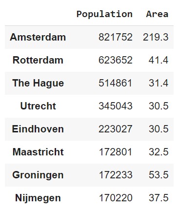
Ascending Sort
We can use the sort_values() method to sort the series.
area = pd.Series({'Rotterdam': 41.4, 'Utrecht': 30.5, 'Amsterdam': 219.3, 'Eindhoven': 30.5, 'The Hague': 31.4})
area.sort_values()
Utrecht       30.5
Eindhoven     30.5
The Hague     31.4
Rotterdam     41.4
Amsterdam    219.3
dtype: float64
Descending Sort
We can also sort the series in descending order using the ascending parameter.
area.sort_values(ascending=False)
Amsterdam    219.3
Rotterdam     41.4
The Hague     31.4
Utrecht       30.5
Eindhoven     30.5
dtype: float64
Inplace Argument
The result of the sort_values() method is a new series, so we need to assign it to a variable if we want to keep it. We can also sort the series in-place using the inplace parameter.
area.sort_values(ascending=False, inplace=True)
print(area)
Amsterdam    219.3
Rotterdam     41.4
The Hague     31.4
Utrecht       30.5
Eindhoven     30.5
dtype: float64
Sorting by Index
We can also sort the series by the index using the sort_index() method.
Rotterdam     41.4
Utrecht       30.5
Amsterdam    219.3
Eindhoven     30.5
The Hague     31.4
dtype: float64
area.sort_index()
Amsterdam    219.3
Eindhoven     30.5
Rotterdam     41.4
The Hague     31.4
Utrecht       30.5
dtype: float64
NaN Values (1)
NaN values are used to represent missing data. We can use the isnull() method to check for NaN values.
Rotterdam     41.4
Utrecht       30.5
Amsterdam    219.3
Maastricht     NaN
Eindhoven     30.5
The Hague     31.4
dtype: float64
print(area.isnull())
Rotterdam     False
Utrecht       False
Amsterdam     False
Maastricht     True
Eindhoven     False
The Hague     False
dtype: bool
NaN Values (2)
We can use the sum() method to count the number of NaN values.
print(area.isnull().sum())
1
Aggregation
Similar to numpy arrays, we can use many aggregation methods on a series.
print(area.sum())
353.1
print(area.mean())
70.62
print(area.std())
83.24209872414319
DataFrame
A DataFrame is a 2-dimensional data structure that can store data of different types in each column. It is similar to a spreadsheet or a SQL table.
DataFrame Components
A DataFrame is made up of three components:
the index, the columns, and the data.
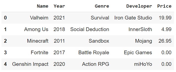
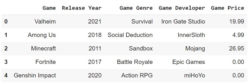
DataFrame Creation (1)
The most straightforward way to create a DataFrame is to pass a dictionary to the pd.DataFrame() constructor.
data = {'Name': ['Valheim', 'Among Us', 'Minecraft', 'Fortnite', 'Genshin Impact'],
        'Year': [2021, 2018, 2011, 2017, 2020],
        'Genre': ['Survival', 'Social Deduction', 'Sandbox', 'Battle Royale', 'Action RPG'],
        'Developer': ['Iron Gate Studio', 'InnerSloth', 'Mojang', 'Epic Games', 'miHoYo'],
        'Price': [19.99, 4.99, 26.95, 0.00, 0.00]}
df = pd.DataFrame(data)
DataFrame Creation (2)
df
DataFrame Creation (3)
We could also pass a list of dictionaries to the pd.DataFrame() constructor.
data = [{'Name': 'Valheim', 'Year': 2021, 'Genre': 'Survival', 'Developer': 'Iron Gate Studio', 'Price': 19.99},
        {'Name': 'Among Us', 'Year': 2018, 'Genre': 'Social Deduction', 'Developer': 'InnerSloth', 'Price': 4.99},
        {'Name': 'Minecraft', 'Year': 2011, 'Genre': 'Sandbox', 'Developer': 'Mojang', 'Price': 26.95},
        {'Name': 'Fortnite', 'Year': 2017, 'Genre': 'Battle Royale', 'Developer': 'Epic Games', 'Price': 0.00},
        {'Name': 'Genshin Impact', 'Year': 2020, 'Genre': 'Action RPG', 'Developer': 'miHoYo', 'Price': 0.00}]
df = pd.DataFrame(data)
DataFrame Creation (4)
We could also pass a list of lists or tuples to the pd.DataFrame() constructor.
data = [['Valheim', 2021, 'Survival', 'Iron Gate Studio', 19.99],
        ['Among Us', 2018, 'Social Deduction', 'InnerSloth', 4.99],
        ['Minecraft', 2011, 'Sandbox', 'Mojang', 26.95],
        ['Fortnite', 2017, 'Battle Royale', 'Epic Games', 0.00],
        ['Genshin Impact', 2020, 'Action RPG', 'miHoYo', 0.00]]
df = pd.DataFrame(data, columns=['Name', 'Year', 'Genre', 'Developer', 'Price'])
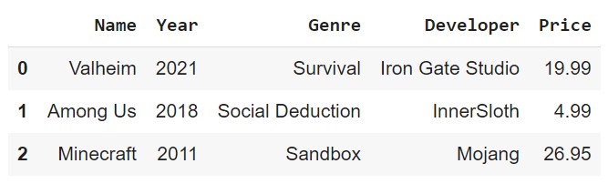
Head and Tail
We can see the first n rows and the last n rows of a DataFrame using the head(n) and tail(n) methods. The default value of n is 5.
df.head(3)
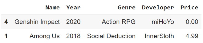
Sample
We can also get a random sample of n rows using the sample(n) method.
df.sample(2)
Get Column Names
We can get the column names of a DataFrame using the columns attribute.
df.columns
Index(['Name', 'Year', 'Genre', 'Developer', 'Price'], dtype='object')
We can also get the column names as a list using the tolist() method.
df.columns.tolist()
['Name', 'Year', 'Genre', 'Developer', 'Price']
Rename Columns
We can rename the columns of a DataFrame using the rename() method.
df.rename(columns={'Name': 'Game', 'Year': 'Release Year', 'Genre': 'Game Genre', 'Developer': 'Game Developer', 'Price': 'Game Price'}, inplace=True)
# or df.columns = ['Game', 'Release Year', 'Game Genre', 'Game Developer', 'Game Price']
df
Column Data Types
We can get the type of a column using the dtypes attribute.
df.dtypes
Game                object
Release Year         int64
Game Genre          object
Game Developer      object
Game Price         float64
dtype: object
df['Game Genre'].dtype
dtype('O')
Retrieve A Column
We can retrieve the values of a column using the [] operator. If the column name is a string with no spaces, we can also use the . operator. The result is a Series.
df['Game']
df.Game
0           Valheim
1          Among Us
2         Minecraft
3          Fortnite
4    Genshin Impact
Name: Game, dtype: object
Retrieve Multiple Columns
We can also retrieve multiple columns. The result is a DataFrame with only the selected columns.
df[['Game', 'Game Genre']]

Get Index
We can get the index of a DataFrame using the index attribute.
df.index
RangeIndex(start=0, stop=5, step=1)
RangeIndex is a special type of index that is used when the index is a sequence of numbers. We can also get the index as a list using the tolist() method.
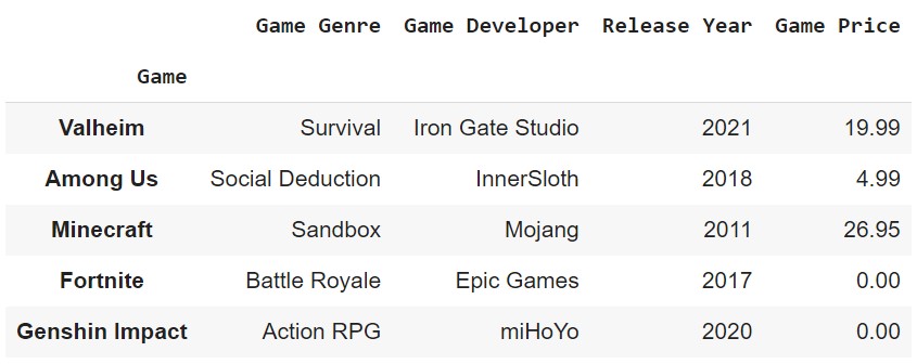
Set Index
We can set the index of a DataFrame using the set_index() method.
df.set_index('Game', inplace=True)
df
Reset Index
We can reset the index of a DataFrame using the reset_index() method. The drop parameter determines whether the old index is dropped or not.
df.reset_index(drop=False, inplace=True)
df
Retrieve A Row
We can retrieve a row using the loc[] or iloc[] operator. The difference between the two is that loc uses the index label, while iloc uses the index position.
df1 = pd.DataFrame([[1, 2], [4, 5], [7, 8]], index=[1, 2, 3], columns=['col1', 'col2'])
df1.iloc[0]
col1    1
col2    2
Name: 1, dtype: int64
df1.loc[0]
KeyError: 0
Slice Rows
We can also slice rows using the loc[] or iloc[] operator. Be aware that the loc operator includes the last index, while the iloc operator does not.
   col1  col2
1     1     2
2     4     5
3     7     8
df1.iloc[1:2]
   col1  col2
2     4     5
df1.loc[1:2]
   col1  col2
1     1     2
2     4     5
Retrieve A Cell
The loc[] and iloc[] operators can also be used to retrieve a cell.
   col1  col2
1     1     2
2     4     5
3     7     8
df1.iloc[0, 0]
1
df1.loc[1, 'col1']
1
Changing Values
We can change the values of a cell after retrieving it.
df1.iloc[0, 0] = 10
   col1  col2
1    10     2
2     4     5
3     7     8
df1.loc[[2, 3], 'col2'] = 100
   col1  col2
1    10     2
2     4   100
3     7   100
Replace Values
We can replace values in a DataFrame using the replace() method.
df1.replace(100, 200)
   col1  col2
1    10     2
2     4   200
3     7   200
DataFrame Info
We can get a summary of a DataFrame using the info() method.
df.info()
<class 'pandas.core.frame.DataFrame'>
RangeIndex: 5 entries, 0 to 4
Data columns (total 5 columns):
 #   Column          Non-Null Count  Dtype
---  ------          --------------  -----
 0   Game            5 non-null      object
 1   Game Genre      5 non-null      object
 2   Game Developer  5 non-null      object
 3   Release Year    5 non-null      int64
 4   Game Price      5 non-null      float64
dtypes: float64(1), int64(1), object(3)
memory usage: 328.0+ bytes
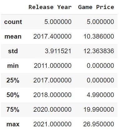
DataFrame Description
We can also get a description of a DataFrame.
df.describe()
Casting Data Types
Similar to NumPy, we can cast the data types of a DataFrame using the astype() method.
df['Game Price'] = df['Game Price'].astype('int64')
Apply Function
Using the apply() method, we can apply a function to a column, row, or DataFrame.
def dollar_to_euro(price):
    return price * 0.92

df['Game Price'] = df['Game Price'].apply(dollar_to_euro)
# Or df['Game Price'] = df['Game Price'].apply(lambda price: price * 0.92)
0    17.48
1     3.68
2    23.92
3     0.00
4     0.00
Name: Game Price, dtype: float64
Map Function
The map() method is similar to the apply() method, but it is used to map values from one set to another.
df['Game Genre'].map({'Action RPG': 0, 'Battle Royale': 1, 'Sandbox': 2, 'Survival': 3, 'Social Deduction': 4})
0    3
1    4
2    2
3    1
4    0
Name: Game Genre, dtype: int64
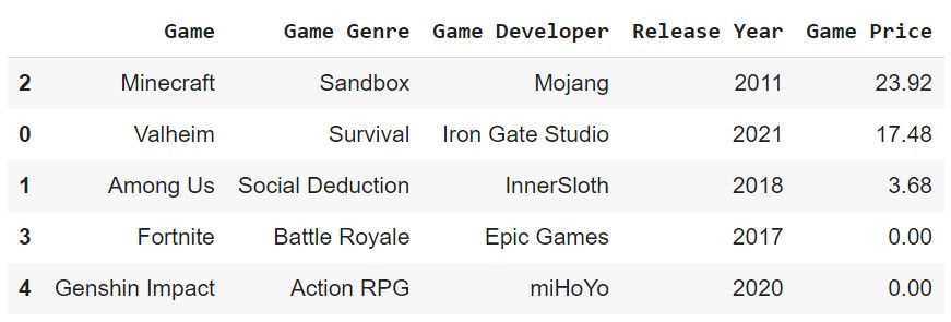
Sorting
We can sort a DataFrame using the sort_values() method. The by parameter determines which column to sort by. The ascending parameter determines whether to sort in ascending or descending order.
df.sort_values(by='Game Price', ascending=False)
inplace=True if you want to replace the original DataFrame.Drop Entries
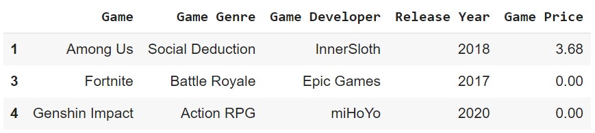
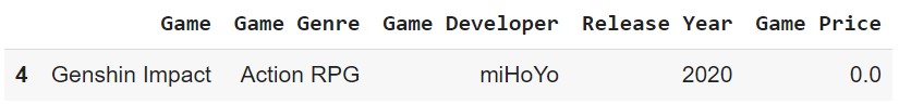
We can drop entries from a DataFrame using the drop() method. The axis parameter determines whether to drop rows or columns. The inplace parameter determines whether to drop the entries in the original DataFrame or not.
df.drop([0, 2], axis=0)
inplace=True if you want to drop the entries in the original DataFrame.Drop Columns
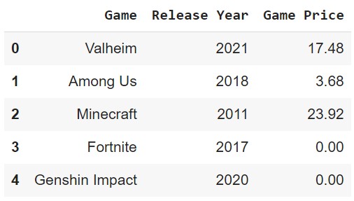
The drop() method can also be used to drop columns.
df.drop(['Game Genre', 'Game Developer'], axis=1)
# Or df.drop(columns=['Game Genre', 'Game Developer'])
inplace=True if you want to drop the columns in the original DataFrame.Filtering (1)
We can use boolean indexing to filter entries.
df['Game Price'] > 20
0    False
1    False
2     True
3    False
4    False
Name: Game Price, dtype: bool
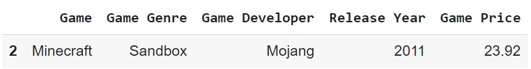
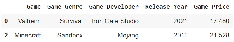
df.loc[df['Game Price'] > 20]
Filtering (2)
We can change the values of retrieved entries.
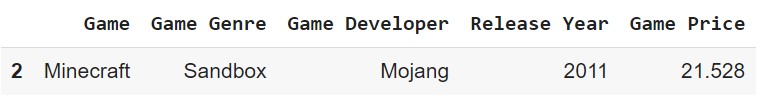
df.loc[df['Game Price'] > 20, 'Game Price'] *= 0.9
Filtering (3)
We can also use the isin() method to check if a value is in a list.
df['Game Genre'].isin(['Survival', 'Battle Royale'])
0     True
1    False
2    False
3     True
4    False
Name: Game Genre, dtype: bool
Filtering (4)
We can use logical operators to filter based on multiple conditions.
df.loc[(df['Game Price'] < 10) & (df['Release Year'] > 2018)]
df.loc[(df['Game Price'] > 20) | (df['Game Genre'] == 'Survival')]
Remove Duplicates
We can remove duplicate entries using the drop_duplicates() method. The keep parameter determines whether to keep the first or last entry.
df2 = pd.DataFrame({'col1': [1, 1, 2, 2, 3, 3, 4, 4],
                    'col2': [1, 1, 2, 2, 3, 3, 4, 4]})
df2.drop_duplicates(keep='first')
   col1  col2
0     1     1
2     2     2
4     3     3
6     4     4
Missing Values (1)
We can check for missing values using the isnull() method.
df3 = pd.DataFrame({'col1': [1, 2, 3, np.nan],
                    'col2': [np.nan, 2, 3, 4]})
df3.isnull()
    col1   col2
0  False   True
1  False  False
2  False  False
3   True  False
Missing Values (2)
We can drop missing values using the dropna() method.
df3.dropna()
   col1  col2
1     2     2
2     3     3
inplace=True if you want to drop the missing values in the original DataFrame.Missing Values (3)
We can fill missing values using the fillna() method.
df3.fillna(0)
   col1  col2
0     1     0
1     2     2
2     3     3
3     0     4
inplace=True if you want to fill the missing values in the original DataFrame.Missing Values (4)
A common way to fill missing values is to use a statistic such as the mean, median, or mode of the column.
df3['col1'].fillna(df3['col1'].mean())
0    1.0
1    2.0
2    3.0
3    2.0
Name: col1, dtype: float64
inplace=True if you want to fill the missing values in the original DataFrame.Date and Time (1)
The to_datetime() method can be used to convert a column to a datetime object.
df4 = pd.DataFrame({'col1': ['2019-08-02', '2020-09-25', '2023-01-03'],
                    'col2': ['2021-12-01 12:00:00', '2020-05-21 04:30:00', '2023-02-04 12:40:00']})
df4['col1'] = pd.to_datetime(df4['col1'])
df4['col2'] = pd.to_datetime(df4['col2'])
        col1                 col2
0 2019-08-02  2021-12-01 12:00:00
1 2020-09-25  2020-05-21 04:30:00
2 2023-01-03  2023-02-04 12:40:00
df4.dtypes
col1    datetime64[ns]
col2    datetime64[ns]
dtype: object
Date and Time (2)
We can extract the year, month, day, hour, minute, and second from a datetime object.
df4['col2'].dt.year
0    2021
1    2020
2    2023
Name: col2, dtype: int64
df4['col2'].dt.minute
0     0
1    30
2    40
Name: col2, dtype: int64
Date and Time (3)
A datetime object can be converted to a string using the strftime() method.
df4['col2'].dt.strftime('%Y-%m-%d')
0    2021-12-01
1    2020-05-21
2    2023-02-04
Name: col2, dtype: object
Date and Time (4)
We can use the timedelta() method to add or subtract a number of days, hours, minutes, or seconds from a datetime object.
        col1                 col2
0 2019-08-02  2021-12-01 12:00:00
1 2020-09-25  2020-05-21 04:30:00
2 2023-01-03  2023-02-04 12:40:00
df4['col2'] + pd.Timedelta(days=1)
0   2021-12-02 12:00:00
1   2020-05-22 04:30:00
2   2023-02-05 12:40:00
Name: col2, dtype: datetime64[ns]
Data File I/O
Pandas can read and write data from a variety of file formats. The most common file formats are CSV, Excel, and JSON.
df.to_csv('data.csv')
df.to_excel('data.xlsx')
df.to_json('data.json')
df = pd.read_csv('data.csv')
df = pd.read_excel('data.xlsx')
df = pd.read_json('data.json')
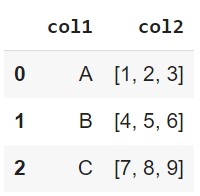
Read JSON Example
{
    "col1": {
        "0": "A",
        "1": "B",
        "2": "C"
    },
    "col2": {
        "0": [1, 2, 3],
        "1": [4, 5, 6],
        "2": [7, 8, 9]
    }
}
df = pd.read_json('data.json')
Write CSV Parameters
The to_csv() method has a number of useful parameters. The following table shows some of the most commonly used parameters.
| Parameter | Description |
|---|---|
index | Write row names (index). Default is True. |
header | Write column names. Default is True. |
sep | Delimiter to use. Default is comma (,). |
Read CSV Parameters
The read_csv() method has a number of useful parameters. The following table shows some of the most commonly used parameters.
| Parameter | Description |
|---|---|
sep | Delimiter to use. Default is comma (,). |
header | Row number to use as the column names. Default is 0. |
index_col | Column number to use as the index. Default is None. |
skiprows | List of row numbers or number of rows to skip at the start of the file. Default is None. |
na_values | Sequence of values to replace with NaN. Default is None. |
parse_dates | Attempt to parse data to datetime. Default is False. |
encoding | Text encoding to use when reading/writing the file. Default is None. |
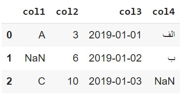
Read CSV Example (1)
col1,col2,col3,col4
A,3,2019-01-01,الف
?,6,2019-01-02,ب
C,10,2019-01-03,N/A
df = pd.read_csv('data.csv', na_values=['N/A', '?'],
                 parse_dates=['col4'], encoding='utf-8')
Read CSV Example (2)
We can also use the read_csv() method to read data from a URL.
imdb = pd.read_csv('https://parsa-abbasi.github.io/slides/pandas/imdb_top_250_movies.csv', index_col='rank')
imdb.head()

Grouping (1)
The groupby() method can be used to group rows of data based on one or more columns. The result of the groupby() method is a DataFrameGroupBy object.
imdb.groupby('year')
<pandas.core.groupby.generic.DataFrameGroupBy object at 0x0000020B1B5B0A90>
Grouping (2)
The DataFrameGroupBy object has a number of useful methods. The following table shows some of the most commonly used methods.
| Method | Description |
|---|---|
count() | Number of non-NA values. |
sum() | Sum of values. |
mean() | Mean of values. |
median() | Arithmetic median of values. |
min() | Minimum. |
max() | Maximum. |
size() | Number of elements in the object. |
Grouping Example (1)
imdb.groupby('year').count()['name']
year
1921    1
1924    1
1925    1
1926    1
1927    1
       ..
2018    4
2019    6
2020    2
2021    2
2022    1
Name: name, Length: 86, dtype: int64
Grouping Example (2)
imdb.groupby('year')['rating'].mean()
year
1921    8.30
1924    8.20
1925    8.10
1926    8.10
1927    8.30
        ...
2018    8.35
2019    8.30
2020    8.30
2021    8.50
2022    8.30
Name: rating, Length: 86, dtype: float64
Transforming
The transform() method can be used to apply a function to each group independently. The result of the transform() method is a Series object.
imdb.groupby('year')['rating'].transform(lambda x: x - x.mean())
rank
1      0.500000
2      0.000000
3      0.500000
4      0.400000
5      0.633333
         ...
246   -0.140000
247   -0.060000
248   -0.166667
249   -0.100000
250   -0.350000
Name: rating, Length: 250, dtype: float64
Merge / Join
The merge() method can be used to join two DataFrame objects. The following table shows some of the most commonly used parameters.
| Parameter | Description |
|---|---|
left | Left `DataFrame` object. |
right | Right `DataFrame` object. |
how | One of left, right, outer, inner, cross. Default is inner. |
on | Column(s) to join on. Must be found in both the left and right `DataFrame` objects. |
left_on | Column(s) in the left `DataFrame` to use as the join keys. |
right_on | Column(s) in the right `DataFrame` to use as the join keys. |
left_index | Use the index from the left `DataFrame` as its join key(s). Default is False. |
right_index | Use the index from the right `DataFrame` as its join key(s). Default is False. |
Merge How Parameter (1)
The following table shows some of the most commonly used values for the how parameter.
| Value | Description |
|---|---|
inner | Use intersection of keys from both `DataFrame` objects. |
left | Use only keys from left `DataFrame` object. |
right | Use only keys from right `DataFrame` object. |
outer | Use union of keys from both `DataFrame` objects. |
cross | Use cartesian product with each row from the left `DataFrame` object being paired with each row from the right `DataFrame` object. |
Merge How Parameter (2)

Inner Join
df1 = pd.DataFrame({'City': ['Amsterdam', 'Tilburg', 'Rotterdam', 'Utrecht'],
                    'Population': [821752, 213310, 623652, 340852]})
df2 = pd.DataFrame({'City': ['Rotterdam', 'Nijmegen', 'Eindhoven', 'Tilburg', 'Utrecht'],
                    'Area': [41.78, 32.61, 213.31, 37.29, 30.93]})
pd.merge(df1, df2, how='inner', on='City')
        City  Population   Area
0    Tilburg      213310  37.29
1  Rotterdam      623652  41.78
2    Utrecht      340852  30.93
df1 and df2 are included in the result.Left Join
df1 = pd.DataFrame({'City': ['Amsterdam', 'Tilburg', 'Rotterdam', 'Utrecht'],
                    'Population': [821752, 213310, 623652, 340852]})
df2 = pd.DataFrame({'City': ['Rotterdam', 'Nijmegen', 'Eindhoven', 'Tilburg', 'Utrecht'],
                    'Area': [41.78, 32.61, 213.31, 37.29, 30.93]})
pd.merge(df1, df2, how='left', on='City')
        City  Population   Area
0  Amsterdam      821752    NaN
1    Tilburg      213310  37.29
2  Rotterdam      623652  41.78
3    Utrecht      340852  30.93
df1 are included in the result, even if they are not present in df2. The missing values are filled with NaN.Right Join
df1 = pd.DataFrame({'City': ['Amsterdam', 'Tilburg', 'Rotterdam', 'Utrecht'],
                    'Population': [821752, 213310, 623652, 340852]})
df2 = pd.DataFrame({'City': ['Rotterdam', 'Nijmegen', 'Eindhoven', 'Tilburg', 'Utrecht'],
                    'Area': [41.78, 32.61, 213.31, 37.29, 30.93]})
pd.merge(df1, df2, how='right', on='City')
        City  Population    Area
0  Rotterdam    623652.0   41.78
1   Nijmegen         NaN   32.61
2  Eindhoven         NaN  213.31
3    Tilburg    213310.0   37.29
4    Utrecht    340852.0   30.93
df2 are included in the result, even if they are not present in df1. The missing values are filled with NaN.Outer Join
df1 = pd.DataFrame({'City': ['Amsterdam', 'Tilburg', 'Rotterdam', 'Utrecht'],
                    'Population': [821752, 213310, 623652, 340852]})
df2 = pd.DataFrame({'City': ['Rotterdam', 'Nijmegen', 'Eindhoven', 'Tilburg', 'Utrecht'],
                    'Area': [41.78, 32.61, 213.31, 37.29, 30.93]})
pd.merge(df1, df2, how='outer', on='City')
        City  Population    Area
0  Amsterdam    821752.0     NaN
1    Tilburg    213310.0   37.29
2  Rotterdam    623652.0   41.78
3    Utrecht    340852.0   30.93
4   Nijmegen         NaN   32.61
5  Eindhoven         NaN  213.31
df1 and df2 are included in the result. The missing values are filled with NaN.Cross Join
df1 = pd.DataFrame({'City': ['Amsterdam', 'Tilburg', 'Rotterdam', 'Utrecht'],
                    'Population': [821752, 213310, 623652, 340852]})
df2 = pd.DataFrame({'City': ['Rotterdam', 'Nijmegen', 'Eindhoven', 'Tilburg', 'Utrecht'],
                    'Area': [41.78, 32.61, 213.31, 37.29, 30.93]})
pd.merge(df1, df2, how='cross')
City_x  Population City_y   Area
       City_x  Population     City_y    Area
0   Amsterdam      821752  Rotterdam   41.78
1   Amsterdam      821752   Nijmegen   32.61
2   Amsterdam      821752  Eindhoven  213.31
3   Amsterdam      821752    Tilburg   37.29
4   Amsterdam      821752    Utrecht   30.93
5     Tilburg      213310  Rotterdam   41.78
6     Tilburg      213310   Nijmegen   32.61
...
df1 and df2 are included in the result. The missing values are filled with NaN.Concatenatination (1)
The concat() function is used to concatenate two or more DataFrames.
df1 = pd.DataFrame({'City': ['Amsterdam', 'Tilburg', 'Rotterdam', 'Utrecht'],
                    'Population': [821752, 213310, 623652, 340852]})
df2 = pd.DataFrame({'City': ['Eindhoven', 'Nijmegen', 'Groningen'],
                    'Population': [223452, 165432, 248563]})
pd.concat([df1, df2])
        City  Population
0  Amsterdam      821752
1    Tilburg      213310
2  Rotterdam      623652
3    Utrecht      340852
0  Eindhoven      223452
1   Nijmegen      165432
2  Groningen      248563
Concatenatination (2)
We can also concatenate DataFrames along the columns.
df1 = pd.DataFrame({'City': ['Amsterdam', 'Tilburg', 'Rotterdam', 'Utrecht'],
                    'Population': [821752, 213310, 623652, 340852]})
df2 = pd.DataFrame({'Area': [41.78, 32.61, 213.31, 37.29, 30.93],
                    'Density': [19857, 6554, 2954, 9123, 10000]})
pd.concat([df1, df2], axis=1)
        City  Population    Area  Density
0  Amsterdam    821752.0   41.78    19857
1    Tilburg    213310.0   32.61     6554
2  Rotterdam    623652.0  213.31     2954
3    Utrecht    340852.0   37.29     9123
4        NaN         NaN   30.93    10000
Manipulating Text Data (1)
The str attribute of a Series provides access to a set of string manipulation methods.
df = pd.DataFrame({'City': ['Amsterdam', 'Tilburg', 'The Hague'],
                   'Province': ['North Holland', 'North Brabant', 'South Holland']})
df['City'].str.upper()
0    AMSTERDAM
1      TILBURG
2    THE HAGUE
Name: City, dtype: object
df['City'].str.lower()
0    amsterdam
1      tilburg
2    the hague
Name: City, dtype: object
Manipulating Text Data (2)
df['City'].str.len()
0    9
1    7
2    9
Name: City, dtype: int64
df['Province'].str.contains('Holland')
0     True
1    False
2     True
Name: Province, dtype: bool
Manipulating Text Data (3)
df['City'].str.replace('The Hague', 'Den Haag')
0    Amsterdam
1      Tilburg
2     Den Haag
Name: City, dtype: object
df['Province'].str.split(' ')
0    [North, Holland]
1    [North, Brabant]
2    [South, Holland]
Name: Province, dtype: object
Correlation
The corr() function is used to compute pairwise correlation of columns.
df = pd.DataFrame({'Population': [821752, 213310, 623652, 340852, 223452, 165432, 248563],
                   'Area': [41.78, 32.61, 213.31, 37.29, 30.93, 32.61, 213.31],
                   'Density': [19857, 6554, 2954, 9123, 10000, 6554, 2954]})
df.corr()
            Population      Area   Density
Population    1.000000  0.197199  0.564658
Area          0.197199  1.000000 -0.602733
Density       0.564658 -0.602733  1.000000
Density and Population is positive, while the correlation between Density and Area is negative. This is because the density of a city is inversely proportional to the area of the city and directly proportional to the population of the city.Resampling (1)
Resampling is a data aggregation task that involves grouping data into time intervals and applying a function to each group.
df = pd.DataFrame({'Date': ['2022-01-01', '2022-01-02', '2022-01-03', '2022-01-04', '2022-01-05', '2022-01-06', '2022-01-07'],
                   'Temperature': [5.3, 3.8, 2.1, 1.2, 0.5, 1.8, 3.1]})
df['Date'] = pd.to_datetime(df['Date'])
df = df.set_index('Date')
Resampling (2)
The resample() function is used to resample the DataFrame.
df.resample('2D').mean()
            Temperature
Date
2022-01-01         4.55
2022-01-03         1.65
2022-01-05         1.15
2022-01-07         3.10
df.resample('M').max()
            Temperature
Date
2022-01-31          5.3
Finishing Up
Thank you for keeping up with me until the end!
If you have any questions or suggestions, please send me an email at parsa.abbasi1996@gmail.com.