Introduction to NumPy

Last updated: March 28, 2023

What is NumPy?

NumPy, short for Numerical Python, is a fundamental library for data analysis and scientific computing in the Python programming language.

Why NumPy? (1)

Multidimensional Arrays: NumPy arrays can have any number of dimensions, which makes it possible to store and manipulate complex data sets.
High Performance: NumPy core is based on a highly optimized C implementation, which means that it can perform mathematical and numerical operations much faster than pure Python.

Why NumPy? (2)

Mathematical Functions: NumPy provides a wide variety of mathematical functions for operations, including statistics, linear algebra, and Fourier Transforms.
Efficient and Fast Computation: NumPy allows for fast and accurate computation through powerful vectorized operations and optimized mathematical functions.

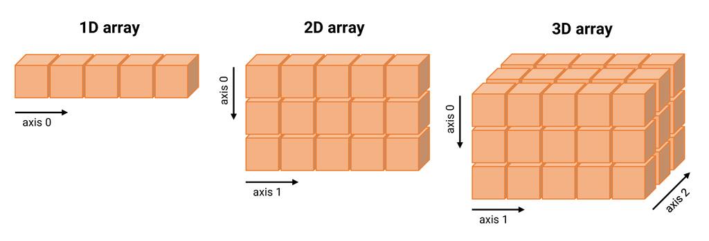
N-dimensional array

One of the key features of NumPy is its N-dimensional array object, or ndarray, which is a fast, flexible container for large datasets in Python.

Note: An ’ndarray’ is a multidimensional, homogeneous array which means that all the elements in the array are of the same type.

Creating a NumPy array (1)

The easiest way to create an ndarray is to use the array() function and pass any sequence-like object (e.g. a list, tuple, or another array) to it.

import numpy as np
data = [1, 2.5, 3.1, 4, 5.6]
arr = np.array(data)

array([1. , 2.5, 3.1, 4. , 5.6])

Creating a NumPy array (2)

import numpy as np
data = [[1, 2, 3, 4], [5, 6, 7, 8]]
arr = np.array(data)

array([[1, 2, 3, 4],
       [5, 6, 7, 8]])

Number of dimensions

We can check the number of dimensions of an array using the ndim attribute.

array([[1, 2, 3, 4],
       [5, 6, 7, 8]])

arr.ndim

Shape of an array

The shape attribute returns a tuple of integers indicating the size of the array in each dimension.

array([[1, 2, 3, 4],
       [5, 6, 7, 8]])

arr.shape

(2, 4)

Size of an array

The size attribute returns the total number of elements of the array.

array([[1, 2, 3, 4],
       [5, 6, 7, 8]])

arr.size

Visualization

Reshaping an array

We can change the shape of an array by using:

arr.reshape(new_shape)

where new_shape is a tuple of integers indicating the new shape of the array.

array([[1, 2, 3, 4],
       [5, 6, 7, 8]])

arr.reshape((4, 2))

array([[1, 2],
       [3, 4],
       [5, 6],
       [7, 8]])

Flattening an array

We can flatten an array by using the flatten method.

array([[1, 2, 3, 4],
       [5, 6, 7, 8]])

arr.flatten()

array([1, 2, 3, 4, 5, 6, 7, 8])

We can also use the ravel or reshape(-1) methods to flatten an array.

Data type (1)

The dtype attribute is an object describing the type of the elements in the array. Unless specified, NumPy tries to infer a good data type for the array that it creates.

array([[1, 2, 3, 4],
       [5, 6, 7, 8]])

arr.dtype

dtype('int64')

Data type (2)

A full list of NumPy data types can be found here.

Type	Type code	Description
`bool`	`?`	Boolean (True or False) stored as a byte
`int8`	`i1`	Byte (-128 to 127)
`int16`	`i2`	Integer (-32768 to 32767)
`int32`	`i4`	Integer (-2147483648 to 2147483647)
`int64`	`i8`	Integer (-9223372036854775808 to 9223372036854775807)
`uint8`	`u1`	Unsigned integer (0 to 255)
`float16`	`f2`	Half precision float: sign bit, 5 bits exponent, 10 bits mantissa
`float32`	`f4`	Single precision float: sign bit, 8 bits exponent, 23 bits mantissa
`float64`	`f8`	Double precision float: sign bit, 11 bits exponent, 52 bits mantissa
`string_`	`S`	Fixed-length ASCII string type (1 byte per character)
`unicode_`	`U`	Fixed-length Unicode type (number of bytes platform specific)
`object`	`O`	Python object type

Data type examples (1)

Boolean

array = np.array([True, False, True], dtype=bool)

array([ True, False,  True])

String

array = np.array(['hello', 'world', 'numpy'], dtype=np.string_)

array([b'hello', b'world', b'numpy'], dtype='|S5')

Data type examples (2)

Unicode

array = np.array([u'سلام',u'بله',u'خیر'], dtype=np.unicode_)

array(['سلام', 'بله', 'خیر'], dtype='<U4')

Object

array = np.array([{"name": "John", "age": 25}, [1, 2, 3], "hello"], dtype=object)

array([{'name': 'John', 'age': 25}, list([1, 2, 3]), 'hello'],
      dtype=object)

Casting data type

You can explicitly cast an array from one dtype to another using ndarray’s astype method.

array = np.array([1, 2, 3, 4, 5])

array([1, 2, 3, 4, 5])

array.astype(np.float64)

array([1., 2., 3., 4., 5.])

Note: Calling astype always creates a copy of the data, even if the new dtype is the same as the old dtype.

Array creation functions (1)

zeros and ones create arrays of 0’s or 1’s, respectively, with a given length or shape. empty creates an array without initializing its values to any particular value.

np.zeros(10)

array([0., 0., 0., 0., 0., 0., 0., 0., 0., 0.])

np.ones((2, 6))

array([[1., 1., 1., 1., 1., 1.],
       [1., 1., 1., 1., 1., 1.]])

np.empty((1, 2))

array([[1., 1.]])

Array creation functions (2)

zeros_like and ones_like create arrays of 0’s or 1’s with the same shape and dtype as a given array.

array = np.array([[1, 2, 3], [4, 5, 6]])

array([[1, 2, 3],
       [4, 5, 6]])

np.zeros_like(array)

array([[0, 0, 0],
       [0, 0, 0]])

np.ones_like(array)

array([[1, 1, 1],
       [1, 1, 1]])

Array creation functions (3)

full creates an array of a given length or shape and fills it with a given value.

np.full((2, 2), 5)

array([[5, 5],
       [5, 5]])

np.full((2, 2), np.pi)

array([[3.14159265, 3.14159265],
       [3.14159265, 3.14159265]])

Array creation functions (4)

arange is an array-valued version of the built-in Python range function. It returns an array instead of a list.

np.arange(10)

array([0, 1, 2, 3, 4, 5, 6, 7, 8, 9])

np.arange(1, 10, 2)

array([1, 3, 5, 7, 9])

Array creation functions (5)

linspace creates an array of evenly spaced values within a given interval.

np.linspace(0, 10, 5)

array([ 0.,  2.5,  5.,  7.5, 10.])

np.linspace(0, 10, 5, endpoint=False)

array([0., 2., 4., 6., 8.])

Array creation functions (6)

eye and identity create square N x N identity matrices. 1’s on the diagonal and 0’s elsewhere.

np.eye(2)

array([[1., 0.],
       [0., 1.]])

np.identity(3)

array([[1., 0., 0.],
       [0., 1., 0.],
       [0., 0., 1.]])

Note: eye is more flexible in creating identity matrices with diagonal shifted by any position (using k parameter), while identity is simpler and faster for creating square identity matrices with diagonal in center.

Array creation functions (7)

random functions create arrays of random values. rand creates an array of the given shape and populates it with random samples from a uniform distribution over [0, 1).

np.random.rand(2, 3)

array([[0.96446011, 0.79026817, 0.76676859],
       [0.21940235, 0.00295188, 0.88539941]])

NaN and infinity

NumPy provides special floating-point values: NaN (not a number) and inf (infinity). NaN is a special value that represents an undefined or unrepresentable value.

array = np.array([1, 2, np.nan, 3, 4, np.inf])

array([ 1.,  2., nan,  3.,  4., inf])

np.isnan(array)

array([False, False,  True, False, False, False])

np.isinf(array)

array([False, False, False, False, False,  True])

Arithmetic operations (1)

Vectorization is the ability of NumPy to perform mathematical computations and array operations on entire arrays without the need to write explicit loops.

Any arithmetic operations between equal-size arrays applies the operation element-wise.

array1 = np.array([1, 2, 3, 4, 5])
array2 = np.array([5, 4, 3, 2, 1])

array1 - array2

array([-4, -2,  0,  2,  4])

array1 * array2

array([5, 8, 9, 8, 5])

Arithmetic operations (2)

Arithmetic operations with scalars propagate the scalar argument to each element in the array.

array1 = np.array([1, 2, 3, 4, 5])

1 / array1

array([1.        , 0.5       , 0.33333333, 0.25      , 0.2       ])

array1 ** 2

array([ 1,  4,  9, 16, 25])

Arithmetic operations (3)

Comparison operators between arrays are also vectorized.

array1 = np.array([1, 2, 3, 4, 5])
array2 = np.array([5, 4, 3, 2, 1])

array1 > array2

array([False, False, False,  True,  True])

array1 == array2

array([False, False,  True, False, False])

Broadcasting

Broadcasting is a powerful technique in NumPy that allows you to perform arithmetic operations between ndarrays of different shapes and sizes.

The basic idea behind broadcasting is to extend smaller arrays to match the shape of larger arrays so that arithmetic operations can be carried out element-wise.

Broadcasting Rule

Two arrays are compatible for broadcasting if for each trailing dimension (i.e. starting from the end), the dimension sizes match or one of them is 1. Broadcasting is then performed over the missing or size 1 dimensions.

array1 = np.array([[0, 0, 0], [1, 1, 1], [2, 2, 2], [3, 3, 3]])
array2 = np.array([1, 2, 3])

array1 + array2

array([[1, 2, 3],
       [2, 3, 4],
       [3, 4, 5],
       [4, 5, 6]])

Broadcasting Example (1)

Broadcasting Example (2)

Broadcasting Example (3)

Broadcasting Value Error

If the arrays have different shapes and the dimension sizes cannot be matched, then a ValueError is raised.

array1 = np.array([[0, 0, 0], [1, 1, 1], [2, 2, 2], [3, 3, 3]])
array2 = np.array([1, 2])

array1 + array2

ValueError: operands could not be broadcast together with shapes (4,3) (2,)

Integer Indexing (1)

Integer indexing allows you to select or change individual elements in an array.

array = np.array([1, 2, 3, 4])

print(array[0])

print(array[[0, 2]])

[1 3]

Integer Indexing (2)

Integer indexing is also used to access elements of a multidimensional array.

array = np.array([[1, 2], [3, 4], [5, 6]])

print(array[0, 0])

print(array[[0, 1], [0, 1]])

[1 4]

Integer Indexing (3)

Integer indexing can also be used to modify elements of an array.

array = np.array([[1, 2], [3, 4], [5, 6]])

array[0, 0] = 10
print(array)

[[10  2]
 [ 3  4]
 [ 5  6]]

Note: array[0, 0] = 10 is equivalent to array[0][0] = 10.

Slicing

Slicing is the process of accessing a specific section of an ndarray object. The pattern for slicing is:

array[start:stop:step]

start is the index of the first element to be included in the slice. Default is 0.
stop is the index of the first element to be excluded from the slice. Default is the last element.
step is the number of elements to skip between elements in the slice. Default is 1.

Slicing Example (1)

array = np.array([1, 2, 3, 4, 5, 6, 7, 8, 9])

print(array[:5])

[1 2 3 4 5]

print(array[2:5])

[3 4 5]

print(array[2:])

[3 4 5 6 7 8 9]

print(array[1:5:2])

[2 4]

Slicing Example (2)

We can also use negative indices to slice an array.

array = np.array([1, 2, 3, 4, 5, 6, 7, 8, 9])

print(array[-5:-1])

[5 6 7 8]

print(array[-5:])

[5 6 7 8 9]

print(array[:-5])

[1 2 3 4]

print(array[-5:-1 :2])

[5 7]

Slicing Example (3)

array = np.arange(10)
arr_slice = array[5:8]
print(arr_slice)

[5 6 7]

arr_slice[:] = 752
print(arr_slice)

[752 752 752]

print(array)

[  0   1   2   3   4 752 752 752   8   9]

Note: arr_slice is a view of array. Any changes made to arr_slice will be reflected in array. If you want a copy of array instead, use array.copy().

Slicing Example (4)

Boolean Indexing (1)

Boolean indexing is used to select elements of an ndarray based on a boolean mask that has the same shape as the ndarray. The boolean mask is usually the result of a comparison operation.

names = np.array(['Bob', 'Joe', 'Will', 'Bob', 'Will', 'Joe', 'Joe'])
data = np.random.randn(7, 4)

print(names == 'Bob')

[ True False False  True False False False]

print(data[names == 'Bob'])

[[-0.85164614 -0.62923217 -1.00937517 -1.28966066]
 [ 0.38158308 -0.06660506 -0.40679032 -2.21044626]]

Boolean Indexing (2)

We can use negation to select elements that do not satisfy a condition.

print(names != 'Bob')

[False  True  True False  True  True  True]

print(data[names != 'Bob'])

[[ 0.39566302 -0.05056332  0.66541337 -0.64857944]
 [-0.56789928 -3.17910369 -0.62682876  1.37407177]
 [-0.52188158  0.81734887 -0.42735326 -0.32799522]
 [ 0.05523974  0.34693793 -0.73075408 -0.61303047]
 [ 0.5012829  -0.42256724  0.47958592  0.24233269]]

Boolean Indexing (3)

We can also combine boolean masks using the & (and) and | (or) operators.

mask = (names == 'Bob') | (names == 'Will')
print(mask)

[ True False  True  True  True False False]

data[mask]

array([[-0.85164614, -0.62923217, -1.00937517, -1.28966066],
       [-0.56789928, -3.17910369, -0.62682876,  1.37407177],
       [ 0.38158308, -0.06660506, -0.40679032, -2.21044626],
       [-0.52188158,  0.81734887, -0.42735326, -0.32799522]])

Boolean Indexing (4)

We can also use boolean indexing to modify elements of an array.

[[-0.85164614 -0.62923217 -1.00937517 -1.28966066]
 [ 0.39566302 -0.05056332  0.66541337 -0.64857944]
 [-0.56789928 -3.17910369 -0.62682876  1.37407177]
 [ 0.38158308 -0.06660506 -0.40679032 -2.21044626]
 [-0.52188158  0.81734887 -0.42735326 -0.32799522]
 [ 0.05523974  0.34693793 -0.73075408 -0.61303047]
 [ 0.5012829  -0.42256724  0.47958592  0.24233269]]

data[data < 0] = 0

array([[0.        , 0.        , 0.        , 0.        ],
       [0.39566302, 0.        , 0.66541337, 0.        ],
       [0.        , 0.        , 0.        , 1.37407177],
       [0.38158308, 0.        , 0.        , 0.        ],
       [0.        , 0.81734887, 0.        , 0.        ],
       [0.05523974, 0.34693793, 0.        , 0.        ],
       [0.5012829 , 0.        , 0.47958592, 0.24233269]])

Conditional Logic

The np.where function is a vectorized version of the ternary expression x if condition else y.

x = np.array([1, 2, 3, 4, 5])
y = np.array([6, 7, 8, 9, 10])

np.where(x > 3, x, y)

array([ 6,  7,  8,  4,  5])

Universal Functions

A universal function (or ufunc for short) is a function that performs element-wise operations on data in ndarrays. They are fast vectorized wrappers for simple functions that take one or more scalar values and produce one or more scalar results.

Ufunc Example (1)

array = np.arange(5)

np.sqrt(array)

array([0.        , 1.        , 1.41421356, 1.73205081, 2.        ])

np.exp(array)

array([ 1.        ,  2.71828183,  7.3890561 , 20.08553692, 54.59815003])

np.square(array)

array([ 0,  1,  4,  9, 16])

Ufunc Example (2)

array1 = np.random.randn(4)
array2 = np.random.randn(4)

print(array1)

[-0.87035484 -0.62430881  0.24429588 -1.56903064]

print(array2)

[-1.22755972 -0.07799901  1.53771294 -0.69276198]

np.maximum(array1, array2)

array([-0.87035484, -0.07799901,  1.53771294, -0.69276198])

np.minimum(array1, array2)

array([-1.22755972, -0.62430881,  0.24429588, -1.56903064])

Other Ufuncs

There are many other ufuncs available in NumPy. You can find a list of them here. Some of the more common ones are:

Function	Description
`np.power`	Raise corresponding elements in arrays to specified power
`np.mod`	Return remainder of division of corresponding elements in arrays
`np.abs`	Return absolute value of corresponding elements in arrays
`np.sign`	Return sign of corresponding elements in arrays
`np.cos`, `np.sin`, `np.tan`	Trigonometric functions
`np.arccos`, `np.arcsin`, `np.arctan`	Inverse trigonometric functions
`np.log`, `np.log10`, `np.log2`	Logarithmic functions
`np.ceil`, `np.floor`	Round up and down to nearest integer

Aggregate Functions

Aggregate functions are functions that operate on an entire array and return a single value. Some of the more common aggregate functions are:

Function	Description
`np.sum`	Sum of all elements in array
`np.mean`	Mean of all elements in array
`np.std`	Standard deviation of all elements in array
`np.var`	Variance of all elements in array
`np.min`, `np.max`	Minimum and maximum of all elements in array
`np.argmin`, `np.argmax`	Indices of minimum and maximum of all elements in array
`np.median`	Median of all elements in array
`np.percentile`	Percentile of all elements in array

You can find a full list here and here.

Aggregation Example (1)

array = np.array([[1, 2, 3], [4, 5, 6]])
array

array([[1, 2, 3],
       [4, 5, 6]])

array.sum()

array.sum(axis=0)

array([5, 7, 9])

array.sum(axis=1)

array([ 6, 15])

Aggregation Example (2)

array([[1, 2, 3],
       [4, 5, 6]])

array.mean()

3.5

array([2.5, 3.5, 4.5])

array.std()

1.707825127659933

array.var()

2.9166666666666665

array.median(axis=1)

array([2., 5.])

Aggregation Example (3)

array([[1, 2, 3],
       [4, 5, 6]])

array.min()

array.max()

array.argmin()

array.argmax()

Concatenation

NumPy arrays can be concatenated using the concatenate function. We can concatenate arrays along the rows or the columns.

array1 = np.array([[1, 2, 3], [4, 5, 6]])
array2 = np.array([[7, 8, 9], [10, 11, 12]])

np.concatenate([array1, array2])

array([[ 1,  2,  3],
       [ 4,  5,  6],
       [ 7,  8,  9],
       [10, 11, 12]])

np.concatenate([array1, array2], axis=1)

array([[ 1,  2,  3,  7,  8,  9],
       [ 4,  5,  6, 10, 11, 12]])

hstack and vstack

NumPy also provides the hstack and vstack functions for concatenating arrays along the rows and columns respectively.

array1 = np.array([[1, 2, 3], [4, 5, 6]])
array2 = np.array([[7, 8, 9], [10, 11, 12]])

np.vstack([array1, array2])

array([[ 1,  2,  3],
       [ 4,  5,  6],
       [ 7,  8,  9],
       [10, 11, 12]])

np.hstack([array1, array2])

array([[ 1,  2,  3,  7,  8,  9],
       [ 4,  5,  6, 10, 11, 12]])

Column Stacking

We can also stack arrays along the columns using the column_stack function.

array1 = np.array([1, 2, 3])
array2 = np.array([4, 5, 6])

np.column_stack([array1, array2])

array([[1, 4],
       [2, 5],
       [3, 6]])

np.vstack([array1, array2])

array([[1, 2, 3],
       [4, 5, 6]])

np.hstack([array1, array2])

array([1, 2, 3, 4, 5, 6])

Splitting

NumPy arrays can be split using the split function. We can split arrays along the rows or the columns.

array = np.array([[1, 2, 3, 4], [5, 6, 7, 8], [9, 10, 11, 12]])

np.split(array, 3)

[array([[1, 2, 3, 4]]),
 array([[5, 6, 7, 8]]),
 array([[ 9, 10, 11, 12]])]

np.split(array, 3, axis=1)

[array([[ 1,  2],
        [ 5,  6],
        [ 9, 10]]),
 array([[ 3,  4],
        [ 7,  8],
        [11, 12]]),
 array([], shape=(3, 0), dtype=int64)]

Methods for Boolean Arrays

NumPy has a number of methods for boolean arrays.

array = np.array([1, 2, 3, 4, 5])

array > 3

array([False, False, False,  True,  True])

(array > 3).sum()

(array > 3).any()

True

(array > 3).all()

False

Sort

NumPy arrays can be sorted inplace using the sort method.

array = np.array([5, 2, 3, 1, 4])
array.sort()

array([1, 2, 3, 4, 5])

array = np.array([[5, 2, 3],
                  [1, 4, 6]])
array.sort(axis=0)

array([[1, 2, 3],
       [5, 4, 6]])

array.sort(axis=1)

array([[1, 2, 3],
       [4, 5, 6]])

Arg Sort

The argsort method returns the indices of the sorted array.

array = np.array([5, 2, 3, 1, 4])
array.argsort()

array([3, 1, 2, 4, 0])

Unique Elements

NumPy has a unique function that returns the unique elements in an array.

array = np.array([1, 1, 2, 2, 3, 3, 4, 4])
np.unique(array)

array([1, 2, 3, 4])

array = np.array([[1, 1], [2, 3]])
np.unique(array)

array([1, 2, 3])

Vectorize method

The vectorize method allows us to apply a function to every element in an array.

array = np.array(['1,000', '2,000', '3,000'])

def my_func(x):
    return int(x.replace(',', ''))
remove_commas = np.vectorize(my_func)
remove_commas(array)

array([1000, 2000, 3000])

remove_commas = np.vectorize(lambda x: int(x.replace(',', '')))
remove_commas(array)

Note: The primary advantage of using vectorize over using a loop (for or while) is that the function's performance is optimized, which makes the operation faster and more efficient.

File Input and Output

We can save and load NumPy arrays to and from disk using the save and load functions.

array = np.array([1, 2, 3, 4, 5])
np.save('my_array', array)

np.load('my_array.npy')

array([1, 2, 3, 4, 5])

array1 = np.array([1, 2, 3, 4, 5])
array2 = np.array([6, 7, 8, 9, 10])
np.savez('my_arrays.npz', a=array1, b=array2)

archive_array = np.load('my_arrays.npz')
archive_array['a']

array([1, 2, 3, 4, 5])

Linear Algebra

NumPy also has a number of functions for linear algebra. These are available in the np.linalg module. Some of the more common ones are:

Function	Description
`np.transpose`	Transpose of matrix (similar to `array.T`)
`np.dot`	Dot product of two arrays
`np.inner`	Inner product of two arrays
`np.matmul`	Matrix multiplication (similar to @ operator)
`np.linalg.inv`	Invert matrix
`np.linalg.det`	Determinant of matrix
`np.linalg.eig`	Eigenvalues and eigenvectors of matrix
`np.linalg.solve`	Solve linear system of equations
`np.linalg.norm`	Norm of vector

You can find a full list of linear algebra functions here.

Linear Algebra Example

array1 = np.array([[1, 2],
                   [3, 4]])
array2 = np.array([[5, 6],
                   [7, 8]])

np.matmul(array1, array2) # or array1 @ array2

array([[19, 22],
       [43, 50]])

np.inner(array1, array2)

array([[17, 23],
       [39, 53]])

np.dot(array1, array2) # or array1.dot(array2)

array([[19, 22],
       [43, 50]])

Note: Check this out if you want to know more about the difference between np.dot and np.matmul.

Pseudorandom Numbers

We saw earlier that we can use the rand function to generate random numbers from a uniform distribution. We can also generate random numbers from other distributions using the random module.

Function	Description
`np.random.rand`	Uniform distribution over [0, 1)
`np.random.randn`	Standard normal distribution
`np.random.randint`	Uniform distribution of integers
`np.random.random`	Uniform distribution over [0, 1)
`np.random.normal`	Normal distribution
`np.random.binomial`	Binomial distribution
`np.random.poisson`	Poisson distribution

Check out the documentation for a full list of functions.

Shuffle

We can use the shuffle function to shuffle the elements of an array.

array = np.arange(10)
np.random.shuffle(array)
array

array([3, 5, 2, 1, 9, 4, 0, 8, 7, 6])

Seed (1)

We can use the seed function to set the seed for the pseudorandom number generator. This is useful for reproducibility. If we set the seed to the same value, we will get the same sequence of random numbers.

np.random.seed(0)

np.random.rand(5)

array([0.5488135 , 0.71518937, 0.60276338, 0.54488318, 0.4236548 ])

np.random.rand(5)

array([0.64589411, 0.43758721, 0.891773  , 0.96366276, 0.38344152])

Note: If you run the above code again, you will get the same sequence of random numbers.

Seed (2)

The np.random use a global random seed. To avoid this, we can use the RandomState class. To avoid global state, you can use RandomState to create a random number generator isolated from others.

rng = np.random.RandomState(1234)

rng.rand(5)

array([0.19151945, 0.62210877, 0.43772774, 0.78535858, 0.77997581])

Datetimes and Timedeltas (1)

Starting with NumPy 1.7, NumPy provides a set of datetime functions that can be used to create datetime64 and timedelta64 objects.

np.datetime64('2018-01-01')

numpy.datetime64('2018-01-01')

np.datetime64('2018-01-01 12:00')

numpy.datetime64('2018-01-01T12:00')

np.array(['2007-07-13', '2006-01-13', '2010-08-13'], dtype='datetime64')

array(['2007-07-13', '2006-01-13', '2010-08-13'], dtype='datetime64[D]')

Datetimes and Timedeltas (2)

np.arange('2005-02', '2005-03', dtype='datetime64[D]')

array(['2005-02-01', '2005-02-02', '2005-02-03', '2005-02-04',
       '2005-02-05', '2005-02-06', '2005-02-07', '2005-02-08',
       '2005-02-09', '2005-02-10', '2005-02-11', '2005-02-12',
       '2005-02-13', '2005-02-14', '2005-02-15', '2005-02-16',
       '2005-02-17', '2005-02-18', '2005-02-19', '2005-02-20',
       '2005-02-21', '2005-02-22', '2005-02-23', '2005-02-24',
       '2005-02-25', '2005-02-26', '2005-02-27', '2005-02-28'],
      dtype='datetime64[D]')

np.datetime64('2009-01-01') - np.datetime64('2008-01-01')

numpy.timedelta64(365,'D')

np.timedelta64(1,'W') / np.timedelta64(1,'D')

7.0

Finishing Up

Thank you for keeping up with me until the end!

If you have any questions or suggestions, please send me an email at parsa.abbasi1996@gmail.com.